Hash Tables

Here starts with a ubiquitous data structure hash table aka. hash map. The raison d’être of hash table is to implement fast searches, i.e. lookups.

12.1 Supported Operations

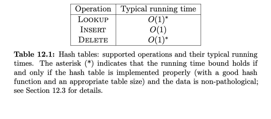
LOOKUP (aka. SEARCH): for a key k, return a pointer to an object in the hash table with key k ( or report that no such object exists)

INSERT: given a new object x, add x to the hash table.

DELETE: for a key k, delete an object with key k from the hash table, if one exists.

When to Use a Hash Table

If your application requires fast lookups with a dynamically changing set of objects, the hash table is usually the data structure of choice.

12.2 Applications

12.2.1 Application: De-duplication

When a new object x with key k arrives:

1. Use LOOKUP to check if the hash table already contains an object with key k.
2. If not, use INSERT to put x in the hash table.

12.2.2 Application: The 2-SUM Problem

Input: An unsorted array A of n integers, and a target integer t.

Goal: Determine whether or not there are two numbers x,y in A satisfying x+y=t.

Attempt 1

This dumb way is implemented by linear research.

for i=1 to n: 
  y := t - A[i]
  // also linear search 
  if A contains y then: 
    return "yes" 
return "no"

or in a sorted array style. Just implement an extra sorting subroutine before run the algorithm.

sort A // using a sorting subroutine. O(nlogn)
for i=1 to n: 
  y := t - A[i] // in this context, it should be O(logn) to search
  if A contains y then:
    return "yes"
return "no"

Here introduce the hash table solution to this question

H := empty hash table
for i = 1 to n:
  INSERT A[i] into H
for i = 1 to n:
  y := t - A[i]
  if H contains y: // using LOOKUP in O(1)
     return "yes"
return "no"

This implementation only take linear time.

12.3 Implementation: High-level Ideas

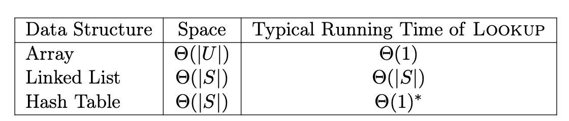
There are 2 straightforward solutions to implement a LOOKUP data structure object.

The asterisk indicates that the running time bound holds iff the hash table is implemented properly and the data is non-pathological.

Hash Function

A hash function $h: U \rightarrow \{0, 1, 2, …, n-1\}$ assigns every key from the $U$ to a pos in an array of length $n$.

However, collisions are inevitable. Because we are trying to throw $|U|$ items into $|S|$ holes.

Collisions: Two keys $k_1$ and $k_2$ from $U$ collide under the hash function $h$ if $h(k_1)=h(k_2)$.

Here introduce a birthday paradox. $n$ people with random birthdays, with each of 366 days of the each year equally likely. at least a 50% chance that 2 people have the same birthday is $n=57$.

So, it’s likely that there are collisions in hash table.

Resolution 1: Chaining

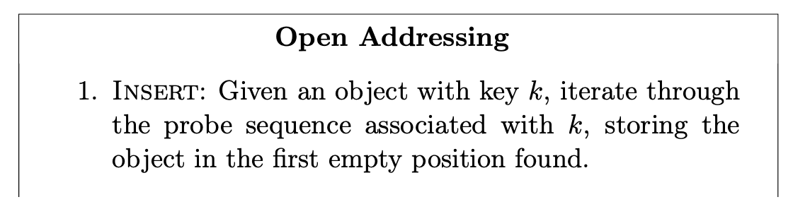
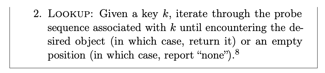
Resolution 2: Open Addressing

Linear Probing

There are several ways to use one or more hash functions to define a probe sequence. This is the simplest one. Simply put, it wraps around the hash table from the beginning to the end.

Double Hashing

Another way is to implement double hashing, which means $h_1(k)=17, h_2(k)=23$, then the first place to check is $k=17$, if it fails, then look up $k=17 + 23$, then $k= 40 + 23$ and so on. The second hash function is changeable from item to item.

Performance

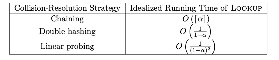
it can be intuitively thought that if a hash table is full of items, then it would be harder for it to check if there’s the desired item, or returning None. So with an appropriate hash table size and hash function, the open addressing achieves. the running time bounds stated in Table 12.1.

What is a good hash function

No matter which collision-resolution strategy we employ, hash table performance degrades with the number of collisions. The best we can hope for is a guarantee that applies to all “non-pathological” data sets.

The good news is that, with a well-crafted hash function, there’s usually no need to worry about pathological data sets in practice.

Random Hash Functions

An extreme approach to decor relating the choice of hash function and the dataset is to choose a random function, meaning a function $h$ where, for each $k \in U$, the value of $h(k)$ is chosen independently and uniformly at random from the array position $\{0,1,2,\cdots, n-1\}$.
Also, the projection relationships has been defined then the function has been implemented.

However, this approach has been proven to be time-consuming also space-consuming.

So what does a good hash function look like?

Good Hash Function

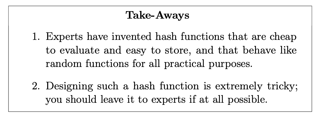
So the random hash function is a desiderata. All we can do is to mimic its performance to create a new hash function.

So a simply-designed the hash function is:

$$ h(k)=(ak+b)\text{mod} n$$

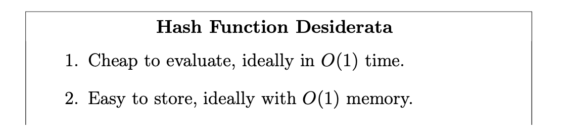
The two most important thing to know about hash function design are:

12.4 Further Implementation Details

Load vs. Performance

We measure the population of a hash table via its load:

$$\text{load of a hash table}=\frac{\text{number of objects stored}}{\text{array length n}}$$

For example, in a chaining hash table, the load is the average population in one of the buckets.

Idealized Performance with Chaining

We want to minimize the $\alpha$, which is the load of a hash table.

Idealized Performance with Open Addressing

with the load is $\alpha$, then there are $1- \alpha$ fraction are empty. With the proof in the geometric random variable, we got the expected value of probing is $\frac{1}{1-\alpha}$.

However, it’s on the basis of the random test. If it based on linear probing, then it would be roughly $\frac{1}{(1-\alpha)^2}$. Because the objects tend to clump together.

 Bloom Filters

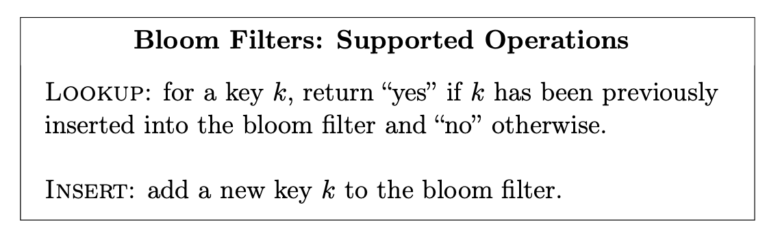
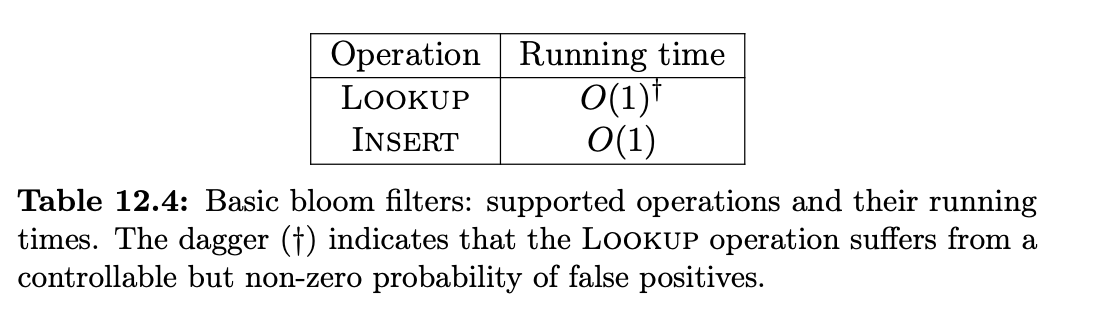
Supported Operations

The raison d’être of a bloom filter is the same as that of hash table: super-fast insertions and lookups. Application compared to hash table: space is at a premium and the occasional error is not a dealbreaker.

Bloom filters require only 8 bits per insertion, compared to 32-bit key or a pointer to an object.

Here are pros and cons between Bloom Filters and Hash Tables:

• Pro: More space efficient
• Pro: Guaranteed constant-time operations for every data set.
• Con: Can’t store pointers to objects.
• Con: Deletions are complicated, relative to a hash table with chaining.
• Con: Non-zero false positive probability.

12.5.2 Applications

Spell checkers: In the 1970s, bloom filters were used to implement spell checkers. People put all the words in the dic into the bloom filter, then check any word flagged as “no”.

Forbidden passwords: this application has been using even today. It’s to keep track of forbidden passwords, which are too common or too easy to guess.

Internet routers: The killer applications of bloom filters is in the core of the Internet. There are many reasons why a router might want to quickly recall what it has seen in the past.  The router might want to look up the source IP address of a packet in the list of blocked IP addresses, or keeping track of the contents of a cache to avoid spurious cache lookups.

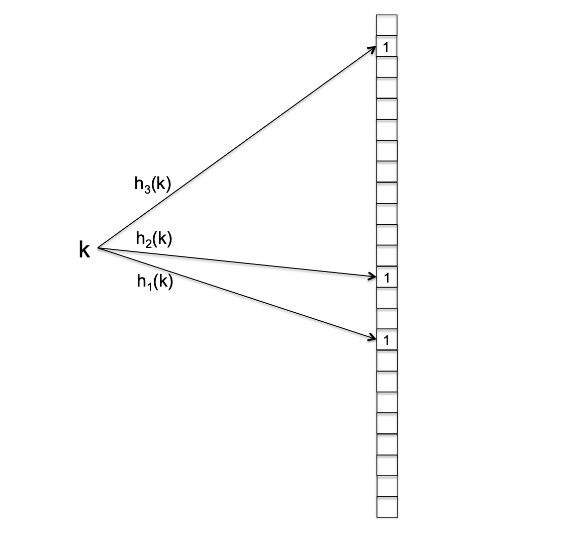
12.5.3 Implementation

For constructing such a filter, what we need are $m$ hash functions, each of them maps the universe $U$ of all possible keys to the set $\{0, 1, 2, \cdots, n-1\}$.  The parameter $m$ is proportional to the number of bits that the bloom filter uses per insertion, and is typically a small constant ( like 5).

Bloom Filter: INSERT( given key k )

for i = 1 to m do
  A[h(k)] = 1

Bloom Filter: LOOKUP (given key k)
for i = 1 to m do
  if A[hi(k)] = 0 then
     return "no"
  return "yes"

IMPORTANT: there are no false negatives cases in the bloom filter. only exists false positive.

Other way, intuitively, as we make the size of the filter bigger, then the number of overlaps between the footprints of keys should decrease, in turn leading to fewer false positives. However, the prime goal of a bloom filter is to save on space. So we want to find a sweet spot where both $n$ and the frequency of false positives are small simultaneously.